Linear regression is a machine learning algorithm in which a best scalar response is established according to the variables. This scalar has the least error and can be used for prediction tasks.
Linear regression works by finding the best values for the variables for equation y = w0 + w1*x, where w0, and w1 are variables. This can be extended to any number of features.
For example: y = w0 + w1*x1 + w2*x2 + … + wn*xn. The best values are found using an algorithm known as gradient descend. But in this post, we will covariance, variance, and mean to find the values for the variables.
We will write the program for the linear regression implementation. We will use python to write this program and we will not use any libraries.
Input
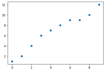
We have the dataset given below. It consists of 2D points.
data = [
        [0,1],
        [1,2],
        [2,4],
        [3,6],
        [4,7],
        [5,8],
        [6,9],
        [7,9],
        [8,10],
        [9,12]
        ]

x = [i[0] for i in data]
y = [i[1] for i in data]

import matplotlib.pyplot as plt
plt.scatter(x,y)
plt.show()
Mean, covariance, and variance function
Now, we will define functions to calculate mean, covariance and variance.
import math

def mean(n):
	return sum(n) / float(len(n))

def covariance(x, mx, y, my):
	covar = 0.0
	for i in range(len(x)):
		covar += (x[i] - mx) * (y[i] - my)
	return covar

def variance(values, mean):
	return sum([(x-mean)**2 for x in values])
Algorithm
Now, we will find the variables using the following code:
x_mean, y_mean = mean(x), mean(y)
w1 = covariance(x, x_mean, y, y_mean) / variance(x, x_mean)
w0 = y_mean - w1 * x_mean
print(w0)
print(w1)
1.6181818181818173
1.1515151515151516
Plotting the line
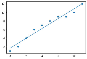
After applying the algorithm, we will plot the predicted line.
import numpy as np
x = np.array(x)
plt.scatter(x,y)
plt.plot(x, w0 + w1*x, linestyle='solid')
plt.show()

Calculating error
We will now find the RMSE error for the predicted line.
def rmse(actual, predicted):
	sum_error = 0.0
	for i in range(len(actual)):
		prediction_error = predicted[i] - actual[i]
		sum_error += (prediction_error ** 2)
	mean_error = sum_error / float(len(actual))
	return (mean_error)**0.5

yPred = [w0 + q*w1 for q in x]
print(rmse(y,yPred))
0.6485414871895709
Predicting the input
Now, we can predict the y value for any input x.
print("Enter the x to classify")
test = [int(i) for i in input().split()]
yNew = w0 + w1 * test[0]
print(yNew)
Enter the x to classify 5 7.375757575757575
That’s it. This is the complete implementation of linear regression.
Complete code
data = [
        [0,1],
        [1,2],
        [2,4],
        [3,6],
        [4,7],
        [5,8],
        [6,9],
        [7,9],
        [8,10],
        [9,12]
        ]

x = [i[0] for i in data]
y = [i[1] for i in data]

import matplotlib.pyplot as plt
plt.scatter(x,y)
plt.show()

import math

def mean(n):
	return sum(n) / float(len(n))

def covariance(x, mx, y, my):
	covar = 0.0
	for i in range(len(x)):
		covar += (x[i] - mx) * (y[i] - my)
	return covar

def variance(values, mean):
	return sum([(x-mean)**2 for x in values])

x_mean, y_mean = mean(x), mean(y)
w1 = covariance(x, x_mean, y, y_mean) / variance(x, x_mean)
w0 = y_mean - w1 * x_mean
print(w0)
print(w1)

import numpy as np
x = np.array(x)
plt.scatter(x,y)
plt.plot(x, w0 + w1*x, linestyle='solid')
plt.show()

def rmse(actual, predicted):
	sum_error = 0.0
	for i in range(len(actual)):
		prediction_error = predicted[i] - actual[i]
		sum_error += (prediction_error ** 2)
	mean_error = sum_error / float(len(actual))
	return (mean_error)**0.5

yPred = [w0 + q*w1 for q in x]
print(rmse(y,yPred))

print("Enter the x to classify")
test = [int(i) for i in input().split()]
yNew = w0 + w1 * test[0]
print(yNew)
Other Machine Learning algorithms:
- Naive Bayes Classification
- K Nearest Neighbors
- Linear Regression
- K Means Clustering
- Apriori Algorithm
- Principal Component Analysis (PCA)
Let us know in the comments if you are having any questions regarding this machine learning algorithm.
And if you found this post helpful, then please help us by sharing this post with your friends. Thank You

